UGRID and LFRic: Polygon mesh intersections¶

I'm aiming to investigate whether it is possible to use the existing python tools to compute intersections of cells definied on the Met Office's LFRic cubesphere. A (possibly out of date but still enlightening) presentation about the LFRic datamodel can also be found here.

I'll start in this notebook with baby steps by using a c12 mesh (6 faces, 12x12 on each face), which is just 864 faces. Naturally, this is several orders of magnitude fewer than the expected mesh of c1024, which is ~6,300,000 faces, but you have to start somewhere, right?

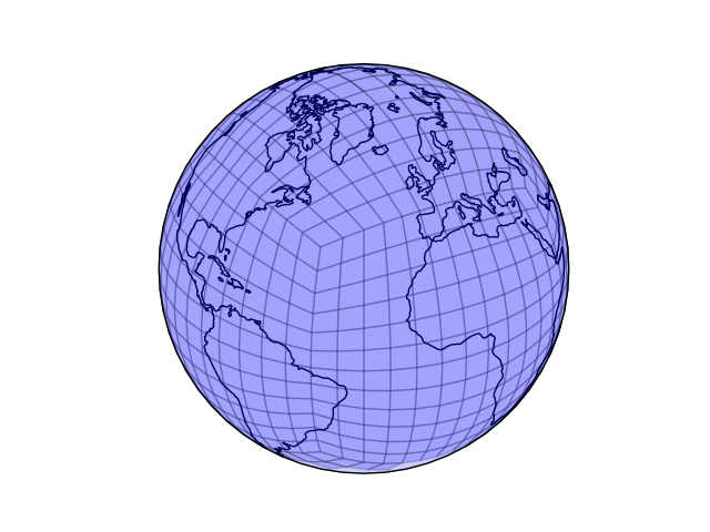
For reference, the LFRic mesh is a cubed-sphere with quadrilateral, approximately equal area, cells.

In [1]:

from IPython.display import Image
Image(filename="cubesphere_ortho.png")

Out[1]:

The go-to tool for geometry based predicates in Python is Shapely, which I'll combine with Cartopy to add a quasi-spherical geometry treatment. I'll not yet move on to real spherical treatment until I know the limitations of these tools for this data.

My ultimate aim is to develop a familiarity with UGRID data so that I can design an Iris based data-model that can be used for easily interacting with the LFRic output.

Here goes...

To start with, I've been given a NetCDF file that uses the UGRID conventions for mesh definition:

In [2]:

!ncdump -h cubedsphere.12x12.fixed.nc

netcdf cubedsphere.12x12.fixed {
dimensions:
        nMesh2_node = 866 ;
        nMesh2_edge = 1728 ;
        nMesh2_face = 864 ;
        Two = 2 ;
        Four = 4 ;
variables:
        int Mesh2 ;
                Mesh2:cf_role = "mesh_topology" ;
                Mesh2:mesh_class = "sphere" ;
                Mesh2:generator_inputs = "edge_cells=12;smooth_passes=0" ;
                Mesh2:long_name = "Topology data of 2D unstructured mesh" ;
                Mesh2:topology_dimension = 2 ;
                Mesh2:node_coordinates = "Mesh2_node_x Mesh2_node_y" ;
                Mesh2:face_node_connectivity = "Mesh2_face_nodes" ;
                Mesh2:edge_node_connectivity = "Mesh2_edge_nodes" ;
                Mesh2:face_edge_connectivity = "Mesh2_face_edges" ;
                Mesh2:face_face_connectivity = "Mesh2_face_links" ;
                Mesh2:face_coordinates = "face_lons face_lats" ;
        int Mesh2_face_nodes(nMesh2_face, Four) ;
                Mesh2_face_nodes:cf_role = "face_node_connectivity" ;
                Mesh2_face_nodes:long_name = "Maps every quadrilateral face to its four corner nodes." ;
                Mesh2_face_nodes:start_index = 1 ;
        int Mesh2_edge_nodes(nMesh2_edge, Two) ;
                Mesh2_edge_nodes:cf_role = "edge_node_connectivity" ;
                Mesh2_edge_nodes:long_name = "Maps every edge to the two nodes that it connects." ;
                Mesh2_edge_nodes:start_index = 1 ;
        int Mesh2_face_edges(nMesh2_face, Four) ;
                Mesh2_face_edges:cf_role = "face_edge_connectivity" ;
                Mesh2_face_edges:long_name = "Maps every quadrilateral face to its four edges." ;
                Mesh2_face_edges:start_index = 1 ;
        int Mesh2_face_links(nMesh2_face, Four) ;
                Mesh2_face_links:cf_role = "face_face_connectivity" ;
                Mesh2_face_links:long_name = "Indicates which other faces neighbour each face." ;
                Mesh2_face_links:start_index = 1 ;
                Mesh2_face_links:flag_values = -1 ;
                Mesh2_face_links:flag_meanings = "out_of_mesh" ;
        double Mesh2_node_x(nMesh2_node) ;
                Mesh2_node_x:standard_name = "longitude" ;
                Mesh2_node_x:long_name = "longitude of 2D mesh nodes." ;
                Mesh2_node_x:units = "radians" ;
        double Mesh2_node_y(nMesh2_node) ;
                Mesh2_node_y:standard_name = "latitude" ;
                Mesh2_node_y:long_name = "latitude of 2D mesh nodes." ;
                Mesh2_node_y:units = "radians" ;
        double face_lats(nMesh2_face) ;
                face_lats:units = "radians" ;
                face_lats:long_name = "Latitudes of face centres" ;
        double face_lons(nMesh2_face) ;
                face_lons:units = "radians" ;
                face_lons:long_name = "Longitudes of face centres" ;
}

Whilst I'm doing this work to ultimately develop a data-model for Iris, interacting with a NetCDF file directly - without any data-model or interpretation - is more easily achieved with XArray.

There seems to be some confusion about what Iris and XArray are. My very simplistic take on the two:

Use XArray if you want to interact with a Python object that looks just like a NetCDF file
Use Iris if you want to interact with a Python object that abstracts the file into standard conventions (CF-conventions)

The key difference being that XArray is very familiar to those comfortable with NetCDF but the lack of standards-based abstraction makes it is easy to write code for one file that does not work with another (for example, when a variable name changes).

There are definitely pros and cons to both, and I hope that one-day we will be able to bridge the gap between the two. For now though, it is fairly easy to convert from one to the other using XArray's xarray.DataArray.to_iris function.

In [3]:

import xarray as xr
ds = xr.open_dataset('cubedsphere.12x12.fixed.nc')
ds

Out[3]:

<xarray.Dataset>
Dimensions:           (Four: 4, Two: 2, nMesh2_edge: 1728, nMesh2_face: 864, nMesh2_node: 866)
Dimensions without coordinates: Four, Two, nMesh2_edge, nMesh2_face, nMesh2_node
Data variables:
    Mesh2             int32 ...
    Mesh2_face_nodes  (nMesh2_face, Four) int32 ...
    Mesh2_edge_nodes  (nMesh2_edge, Two) int32 ...
    Mesh2_face_edges  (nMesh2_face, Four) int32 ...
    Mesh2_face_links  (nMesh2_face, Four) int32 ...
    Mesh2_node_x      (nMesh2_node) float64 ...
    Mesh2_node_y      (nMesh2_node) float64 ...
    face_lats         (nMesh2_face) float64 ...
    face_lons         (nMesh2_face) float64 ...

In [4]:

import numpy as np

xs, ys = np.rad2deg(ds['Mesh2_node_x']), np.rad2deg(ds['Mesh2_node_y'])

Now, let's get those faces as geometries:

In [5]:

import shapely.geometry as sgeom

def lfric_geoms(ds):
    faces = ds['Mesh2_face_nodes']
    offset = faces.attrs.get('start_index', 0)

    if offset:
        faces -= offset
        faces.attrs['start_index'] = 0

    for face in faces:
        geom = sgeom.Polygon([(xs[i], ys[i]) for i in face])
        yield geom

In [6]:

mesh_geoms = list(lfric_geoms(ds))
len(mesh_geoms)

Out[6]:

So for those 864 faces, how long is it taking us to construct them?

In [7]:

%timeit list(lfric_geoms(ds))

3.84 s ± 881 ms per loop (mean ± std. dev. of 7 runs, 1 loop each)

Let's dive straight in and use cartopy to get a land geometry. There are so many ways of doing this (looking at you GeoPandas), but here is one I wrote a few years ago that still holds up:

In [8]:

import cartopy.io.shapereader as shpreader

shpfilename = shpreader.natural_earth(
    resolution='110m', category='cultural', name='admin_0_countries')
countries = list(shpreader.Reader(shpfilename).records())

[Australia] = [country for country in countries
               if country.attributes['NAME'] == 'Australia']
AU_geom = Australia.geometry

So I intend to check the intersection of this Australia geometry with the mesh. Whenever you do repeated intersection calculations with shapely, you should consider "preparing" it to factorise out some of the initialisation

In [9]:

from shapely.prepared import prep

AU_prep = prep(AU_geom)

In [10]:

%timeit [AU_prep.intersects(cell) for cell in mesh_geoms]

11.9 ms ± 1.24 ms per loop (mean ± std. dev. of 7 runs, 100 loops each)

In [11]:

AU_geoms = [cell for cell in mesh_geoms
            if AU_prep.intersects(cell)
            # Pick out only small-ish cells for now. More detail later on...
            if cell.area < 2000]
len(AU_geoms)

Out[11]:

So let's take a look at these matching geometries... cartopy is the go-to tool here.

I'll also get hold of matplotlib and use the interactive backend so that I can interact with the figure while developing in the notebook.

In [12]:

import cartopy.crs as ccrs
import matplotlib as mpl
import matplotlib.pyplot as plt

mpl.rcParams['figure.figsize'] = (4, 4)

%matplotlib notebook

This little utility function is a god-send. I should probably get it into cartopy...

In [13]:

def set_extent_from_geom(ax, geom):
    x0, y0, x1, y1 = geom.bounds
    ax.set_extent([x0, x1, y0, y1], ccrs.Geodetic())

OK, all ducks in a row, now plot the mesh cells that we found to intersect with Australia.

In [14]:

plt.figure()
pc_180 = ccrs.PlateCarree(central_longitude=180)
ax = plt.axes(projection=pc_180)
ax.add_geometries(AU_geoms, ccrs.PlateCarree(),
                  facecolor='blue', edgecolor='k', alpha=0.3)
set_extent_from_geom(ax, AU_geom.buffer(30))
ax.coastlines();

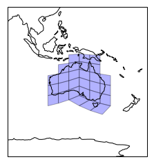
This is a good start. Let's do this on a global scale and produce a land-sea mask.

In [15]:

from shapely.ops import unary_union

shpfilename = shpreader.natural_earth(resolution='110m',
                                      category='physical',
                                      name='land')

land = unary_union(list(shpreader.Reader(shpfilename).geometries()))
# There is a problem with this geometry, so the old "buffer it by 0"
# trick should fix it up for us. 
land = land.buffer(0)
land

Out[15]:

So how many of these mesh cells intersect with land?

In [16]:

land_prep = prep(land)
land_cells = [cell for cell in mesh_geoms
              if land_prep.intersects(cell)]
print(len(land_cells))

This seems a little low. Let's take a look:

In [17]:

plt.figure()
ax = plt.axes(projection=ccrs.PlateCarree())

plt.title('Land geometries')
ax.add_geometries(land_cells, ccrs.PlateCarree(),
                  facecolor='blue', edgecolor='k', alpha=0.3)
ax.coastlines();

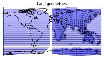
The problem is that some geometries don't back project correctly to a projected space such as plate carree. Until we have spherical geometries, this is always going to be painfull.

Let's leave the painfull cells out for now..

In [18]:

def drop_large(geoms, area):
    """Generator of geometries that have an area below the given value."""
    for geom in geoms:
        if geom.area < area:
            yield geom

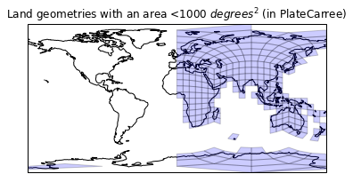
plt.figure()
ax = plt.axes(projection=ccrs.PlateCarree())
plt.title('Land geometries with an area <1000 $degrees^2$ (in PlateCarree)')
ax.add_geometries(drop_large(land_cells, 1000),
                  ccrs.PlateCarree(),
                  facecolor='blue', edgecolor='k', alpha=0.3)
ax.coastlines();

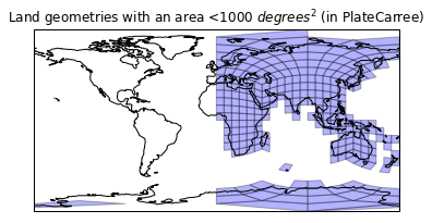
Clearly we have had a bit of sucess here, but we must be suffering from a value range of [0,360] and [-180,180]. Our land geometry lies within [-180, 180], but our mesh doesn't:

In [19]:

def multipoly_geom_xlimit(multipoly):
    if not multipoly.geoms:
        raise ValueError('Not a multipolygon')
    
    xmin = min([min(geom.exterior.coords)[0] for geom in multipoly.geoms])
    xmax = max([max(geom.exterior.coords)[0] for geom in multipoly.geoms])
    return xmin, xmax

print('Land min: {}; max: {}'.format(*multipoly_geom_xlimit(land)))
print('Cells min: {}; max: {}'.format(float(xs.min()), float(xs.max())))

Land min: -180.0; max: 180.00000000000014
Cells min: -0.0; max: 352.5000000475477

In projected space these ranges are critical, and require a reprojection of one or the other geometry. Let's re-project the land geometry, as there are fewer of those. In truth though, I usually try to normalise to [-180, 180].

The trick is to convert the geometry into a PlateCarree with a central longitude at the antimeridian, and then to add 180 to the values to get us back to longitude and latitudes.

In [20]:

pc_180 = ccrs.PlateCarree(central_longitude=180)

# Instead of the geometry in lon/lat, let's project it to lon+180/lat.
land_180 = pc_180.project_geometry(land, ccrs.PlateCarree())

# Same trick as before - try to make this a valid geometry.
land_180 = land_180.buffer(0)

# Finally, translate the projected lon+180/lat geometry back to lon/lat.
import shapely.affinity

land_180 = shapely.affinity.translate(land_180, xoff=180)

land_180

Out[20]:

Let's double check this geometry is as expected:

In [21]:

print('Land_180 min: {}; max: {}'.format(*multipoly_geom_xlimit(land_180)))

Land_180 min: 0.0; max: 360.0

So using the original mesh cells in the range [0, 360] and our projected land in the range [0, 360], let's compute the intersections!

In [22]:

land_180_prep = prep(land_180)
land_180_geoms = [cell for cell in mesh_geoms
                  if land_180_prep.intersects(cell)]
print(len(land_180_geoms))

Great! We have more matching cells than we did before!

In [23]:

def draw_mesh(ax, geoms):
    # Note: Writing functions that take the axes as an argument is a
    # recommended paragdim. It allows easy subplot creation ;)
    ax.coastlines()
    ax.add_geometries(
        geoms,
        ccrs.PlateCarree(),
        facecolor='blue', edgecolor='k', alpha=0.2)

plt.figure()
ax = plt.axes(projection=ccrs.PlateCarree())
plt.title('Land geometries with an area <1000 $degrees^2$ (in PlateCarree)')

draw_mesh(ax, drop_large(land_180_geoms, 1000));

Nope, that wasn't it. Must be an issue with the faces on the western portion of the projection.

Turns out, cartopy doesn't handle the PlateCarree geometries that are greater than 180. This does surprise me, which itself is a surprise given I wrote cartopy. For now, let's just move those cells we've identified back by 360 degrees if they are too far over.

In [24]:

def fixup_wraparound_geoms(geoms):
    # If a cell is over 180, move it back 360.
    for geom in geoms:
        if max(geom.exterior.coords)[0] > 180:
            yield shapely.affinity.translate(geom, xoff=-360)
        else:
            yield geom

In [25]:

plt.figure()
ax = plt.axes(projection=ccrs.PlateCarree())
plt.title('Land cells with an area $<1000 degrees^2$ in PlateCarree')

draw_mesh(ax,
          fixup_wraparound_geoms(drop_large(land_180_geoms, 1000)));

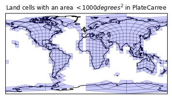
More progress. Notice that we are identifying corner cells here, so no worries there!

Now let's look at the antimeridian issue with the stripe through Europe and Africa missing.

I guess at the dateline there are geometries that have a wraparound which has impacted their geometry orientation (that was probably why we were getting those really wide cells in our first plot, and why filtering large area geometries has been an effective way of removing them). This is probably a bug with the data, as it does state that the geometry should be CCW (on the sphere).

Observation: all UGRIDs are implicitly spherical if they are global and nodes are shared between geometries that cross the antimeridian.

This is getting a bit manual. Instead of playing whack-a-mole with these mesh geometries, let's try projecting the mesh the cells into plate carree from a geodetic coordinate system using cartopy.

That will make some of the cells have many more than 4 nodes, but it will be much more representative of their shape in PlateCarree. It seems highly unlikely that this approach will scale beyond the c12 mesh though...

In [26]:

def project_from_geodetic(geoms):
    pc = ccrs.PlateCarree()
    geod = ccrs.Geodetic()
    for geom in geoms:
        yield pc.project_geometry(geom, geod)

mesh_geoms_prj = list(project_from_geodetic(lfric_geoms(ds)))

How long did that take? Remember that the original lfric_geoms call was ~3s:

In [27]:

%timeit mesh_geoms_prj = list(project_from_geodetic(lfric_geoms(ds)))

6.2 s ± 899 ms per loop (mean ± std. dev. of 7 runs, 1 loop each)

~4.5s is far better than I thought it would be, if I'm honest.

OK, let's use these nicely projected geometries and plot them all:

In [28]:

def draw_mesh(ax, geoms):
    # Note: Writing functions that take the axes as an argument is a
    # recommended paragdim. It allows easy subplot creation ;)
    ax.coastlines()
    ax.add_geometries(
        geoms,
        ccrs.PlateCarree(),
        facecolor='blue', edgecolor='k', alpha=0.2)

plt.figure()
draw_mesh(plt.axes(projection=ccrs.PlateCarree()),
          mesh_geoms_prj)
plt.title('Land cells with an area $<1000 degrees^2$ in PlateCarree');

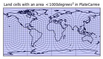
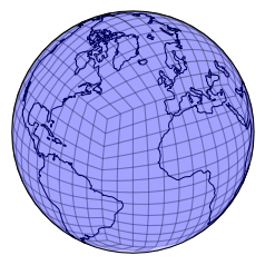
Wowzers, that seems to have done the trick nicely. Let's look at this in a few different ways:

In [29]:

plt.figure()
draw_mesh(plt.axes(projection=ccrs.Orthographic(-30, 30)),
          mesh_geoms_prj);

In [30]:

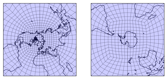
plt.figure(figsize=[10, 5])
ax1 = plt.subplot(1, 2, 1, projection=ccrs.NorthPolarStereo())
ax2 = plt.subplot(1, 2, 2, projection=ccrs.SouthPolarStereo())

for ax in [ax1, ax2]:
    draw_mesh(ax, mesh_geoms_prj)
    lim = 1e7
    ax.set_extent([-lim, lim, -lim, lim], ccrs.SouthPolarStereo())

And finally, do these nicely projected mesh cells actually function as we expect when it comes to land intersection?

In [31]:

land_geoms = [cell for cell in mesh_geoms_prj
              if land_prep.intersects(cell)]
print(len(land_geoms))

In [32]:

plt.figure()
draw_mesh(plt.axes(projection=ccrs.PlateCarree()),
          land_geoms)
plt.title('All land geoms in PlateCarree');

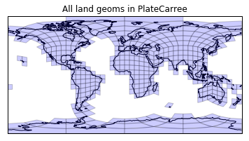
Success! The indices of these cells can be back computed fairly easily:

In [33]:

land_geoms_ids = [id(geom) for geom in land_geoms]
land_mask = np.array([id(geom) in land_geoms_ids for geom in mesh_geoms_prj])

print('n-faces: {}, n-land-faces: {}'.format(land_mask.size, land_mask.sum()))

ds['face_lats'][land_mask]

n-faces: 864, n-land-faces: 423

Out[33]:

<xarray.DataArray 'face_lats' (nMesh2_face: 423)>
array([ 0.709339,  0.717838,  0.717838, ..., -0.779728, -0.813979, -0.836692])
Dimensions without coordinates: nMesh2_face
Attributes:
    units:      radians
    long_name:  Latitudes of face centres

What do the land cells look like on a South polar stereo plot?

In [34]:

plt.figure()
draw_mesh(plt.axes(projection=ccrs.SouthPolarStereo()),
          land_geoms)
plt.title('All land geoms in South Polar Stereographic')

lim = 1.6e7
plt.gca().set_extent([-lim, lim, -lim, lim], ccrs.SouthPolarStereo());

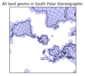
Looks rather splendid. Remember, the containment testing happened in PlateCarree space (poles, wraparounds and all), yet we seem to have got away with this working even for Antarctica.

Conclusion¶

The approach of projecting the spherical/geodetic geometries into PlateCarree with cartopy works.

I do not expect this approach to scale to millions of cells (as is the case for c1024 - a 1024x1024x6 mesh of faces), but I will put metrics on that in a follow-up notebook. The scaling issue comes from the fact that Shapely is operating at the python level, and creating that many objects of any kind is going to be slow. This is doubly true if we are having to project those shapely geometries through cartopy (another Python layer).

What's more, it seems unlikely that we really want to visualise the results in this way for a c1024 mesh. There are more efficient rasterisation techniques (e.g. AGG and datashader) that will work very effectively and provide equivalent fidelity to a figure (but still not render all ~6,200,00 faces in the figure itself).

The wraparound and poles are going to consistently prove to be problematic unless we can handle truly spherical geometries. Cartopy gets us close, but there is no good non-spherical representation of geometries that can be done with GEOS/Shapely.

Is S2 the solution to this perhaps? Can that be made to scale? Does ESMF have a trick up its sleve for containment testing on the sphere?

Investigating containment testing on LFRic's cubedsphere

UGRID and LFRic: Polygon mesh intersections¶

Conclusion¶