
I often deal with huge gridded datasets which either stretch or indeed are beyond the limits of my computer's memory. In the past I've implemented a couple of workarounds to help me handle this data to extract meaningful analyses from them. One of the most intuitive ways of reducing gridded datasets is through indexing/slicing and in this regard netcdf4-python's excellent ability to slice subsets of a larger NetCDF file is invaluable. The problem with the netcdf4-python implementation is that this capability is only available if you have NetCDF files, and doing any analysis on the data involves loading all of the data into memory in the form of a numpy array.
That is where biggus steps in.
import biggus
In this article I will cover some of the basic biggus classes and demonstrate its use in visualising part of an array which is an order of magnitude larger than my machine's memory.
A very convenient and extremely large dataset is the map tile images made available via the folks over at mapquest.com. As some very rudimentary background, the map tiles are split into distinct zoom levels with each zoom level z having 2**z by 2**z images of 256x256 pixels each. So at zoom level 0, there is 1 image to represent the whole globe, with a resolution of 256x256 pixels. At zoom level 1 that turns into 2x2 images, with a combined resolution of 512x512. In the case of these images there is also an RGB channel, which means at zoom level 9 we have a combined resolution image of shape (131072, 131072, 3).
Ok, lets start by implementing a class which represents a given x, y, z map tile. We will also add a __getitem__ method which actually retrieves the data from the web server.
import io
import urllib

import numpy as np
import PIL.Image


class TileLoader(object):
    URL_TEMPLATE = 'http://otile1.mqcdn.com/tiles/1.0.0/sat/{z}/{x}/{y}.jpg'

    def __init__(self, x, y, z):
        self.xyz = x, y, z
        #: A cached version of the array that is downloaded.
        self._cached_array = None

        # The required attributes of a "concrete" array, according
        # to biggus, are 'ndim', 'dtype', and 'shape'.
        self.ndim = 3
        self.dtype = np.uint8
        self.shape = (256, 256, 3)

    def __getitem__(self, slices):
        # Implement the getitem/slicing interface which is the interface needed for biggus to create numpy arrays.
        if self._cached_array is None:
            print 'Downloading tile x={} y={} z={}'.format(*self.xyz)
            url = self.URL_TEMPLATE.format(x=self.xyz[0], y=self.xyz[1], z=self.xyz[2])
            tile_fh = urllib.urlopen(url)
            image_file = io.BytesIO(tile_fh.read())
            self._cached_array = np.array(PIL.Image.open(image_file))
        return self._cached_array[slices]
A TileLoader instance can now be created by passing just the x, y, z coordinates of the tile which is of interest. Notice how the data isn't actually loaded until we ask for it with the index notation.
defered_img = TileLoader(x=1, y=2, z=3)
print defered_img[...].shape
print defered_img[::5, 10:35, 0].shape
So far this hasn't required any Biggus specific code, but using this new TileLoder class we can go ahead and create a biggus.ArrayAdapter instance.
import biggus
img = biggus.ArrayAdapter(TileLoader(x=15, y=10, z=5))

print img
sub_img = img[::5, 10:35, 0]
print sub_img
Notice how no "Downloading tile..." message has been printed, yet the correct shape is calculated for the indexed sub-image. This is because biggus helps us to defer the actual data loading step until the data is required and the Array.ndarray() method is called.
sub_img_array = sub_img.ndarray()
print type(sub_img_array), sub_img_array.shape
So we can now arbitrarily index any sized array and the data is not realized until we actually request the data. This is generally the paradigm in Biggus and it allows one to build up complex operations on arrays without needing access to all of the data at once.
Whilst in this example we've still had to load the full 256x256 image before indexing it (see the __getitem__ implementation above), we could implement some clever image loader which picks off the appropriate data from disk. In truth an image of 256x256 is so small that we probably don't need to worry about implementing such a tricky low level data reader in this case, but if you are using netcdf4-python with massive variables then being able to read only the sections of data which are requested becomes invaluable.
Now that we can create biggus.Array instances (biggus.ArrayAdapter is a subclass of biggus.Array) we can use some of its more interesting features. One of the really interesting classes in biggus is LinearMosaic (which again is a biggus.Array subclass) - this class allows one to join together a list of homogeneous biggus.Array instances to form a bigger array.
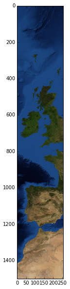
Lets create a biggus.LinearMosaic to represent a column of map tiles at zoom level 5, just to the west of the Greenwich meridian (x=15 at z=5):
arrays = [biggus.ArrayAdapter(TileLoader(x=15, y=y, z=5)) for y in xrange(2 ** 5)]
col = biggus.LinearMosaic(arrays, axis=0)
print col.shape
We can go ahead and slice a subset of the big column of images and visualise the resulting ndarray. Notice how only the necessary images from the 32 image mosaic are actually downloaded.
import matplotlib.pyplot as plt

smaller_column = col[2000:3500]
plt.figure(figsize=(3, 10))
plt.imshow(smaller_column.ndarray())
The biggus.LinearMosaic will take any biggus.Array instances in its mosaic, including other biggus.LinearMosaic instances.
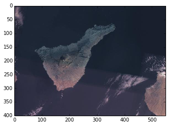
Lets go ahead an make a horizontal mosaic of column mosaics to represent the whole z=9 dataset (that's 2^18 tiles at a resolution of 256x256 each).
def tile_array(z):
    columns = []
    for x in xrange(2 ** z):
        column = [biggus.ArrayAdapter(TileLoader(x=x, y=y, z=z)) for y in xrange(2 ** z)]
        columns.append(biggus.LinearMosaic(column, axis=0))
    return biggus.LinearMosaic(columns, axis=1)

z9 = tile_array(z=9)
print z9.shape
Just in case you were wondering whether you could actually create a numpy array of this size in memory, the answer is only if you are on a machine with at least 48GB of contiguous memory:
def sizeof_fmt(num):
    for x in ['bytes','KB','MB','GB']:
        if num < 1024.0:
            return "%3.1f%s" % (num, x)
        num /= 1024.0
    return "%3.1f%s" % (num, 'TB')

def sizeof_array(a):
    return sizeof_fmt(a.dtype().itemsize * np.prod(a.shape))

print sizeof_array(z9)
Again, we can easily visualise a subset of this large array by using the numpy indexing notation.
smaller_img = z9[54600:55000, 59300:59850]
plt.imshow(smaller_img.ndarray())
Note, this is not a tutorial on spatial extraction of data - there are better ways to extract specific regions of big images than using the pixel index, but that is beyond the scope of this notebook.
So far, we've had to index the biggus.Array in order to pass the data through to matplotlib for visualisation, but wouldn't it be better if we made matplotlib index the array as appropriate for the viewing pane? That way we could pan and zoom on this huge array whilst under the hood, just the parts of the data that need loading actually are.
Fortunately, with a bit of jiggling of the underling matplotlib code this is relatively easy to achieve. The following code block will modify some of the matplotlib internals so that we can go ahead and add the z9 image array as an image to matplotlib and ultimately pan and zoom on that data. Feel free to skip the details of the next code block:
import matplotlib.image as mimg
import matplotlib._image as _image


class AxesBiggusImage(mimg.AxesImage):
    """Subclasses AxesImage to support biggus.Array instances."""
    def set_data(self, A):
        self._A = A

        if (self._A.dtype != np.uint8 and
            not np.can_cast(self._A.dtype, np.float)):
            raise TypeError("Image data can not convert to float")

        if (self._A.ndim not in (2, 3) or
            (self._A.ndim == 3 and self._A.shape[-1] not in (3, 4))):
            raise TypeError("Invalid dimensions for image data")

        self._imcache = None
        self._rgbacache = None
        self._oldxslice = None
        self._oldyslice = None


def frombyte(image, *args, **kwargs):
    """Override frombyte to handle biggus.Array instances."""
    if isinstance(image, biggus.Array):
        image = image.ndarray()
    return _image.frombyte_orig(image, *args, **kwargs)

_image.frombyte_orig = _image.frombyte
_image.frombyte = frombyte
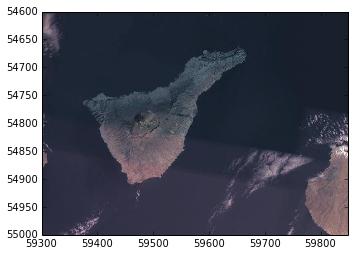
Now for the magic. If you are running this notebook with an interactive matplotlib backend (which I encourage you to try) the following code will produce a standard matplotlib figure with an image of our zoom level 9 data (centered at Tenerife in the Canary Islands) which you can interactively pan and zoom in the same way as you can for any other matplotlib figure - the key difference is that the image that you are viewing is far larger than most machines could possibly hold in memory and therefore only the tiles which are currently being displayed are actually being downloaded from the server. [Note: This has been tested with v1.3.0 of matplotlib]
import matplotlib.pyplot as plt


ax = plt.axes(aspect=1)
im = AxesBiggusImage(ax, origin='upper')
im.set_data(z9)
ax.images.append(im)

plt.xlim(59300, 59850)
plt.ylim(55000, 54600)

plt.show()
In summary, I've shown Biggus' easy to implement biggus.ArrayAdapter interface which gives us a familiar numpy-like interface to any data fit for a numpy array, with the added benefit that combined with off the shelf tools such as the python4-netcdf Variable objects, can quickly make deferred data analysis workflows a reality. The biggus.LinearMosaic allows you to easily build up concatenations of biggus.Arrays (including other biggus.LinearMosaic) instances to form arrays far bigger than could be held in RAM, and allows one to index the data arrays to get hold of smaller, more manageable subsets of the super array. Finally I demonstrated the prospect that matplotlib could one day handle biggus.Array instances without ever needing to read in data that it doesn't ultimately visualise.
Whilst biggus is still very much in its infancy (there is no docs and just a handfull of tests at this point), there is even more to biggus that I haven't discussed here - one very exciting prospect is its ability to do whole dataset operations (such as mean, stddev etc.) without ever needing to allocate all of the memory that the larger array represents - with the added prospect that these operations will become multi-threaded and potentially quicker than the standard numpy operations. In my next post on http://pelson.github.io I will try to cover some of these operations on massive datasets and compare the performance with other tools currently available.
Do you deal with arrays of data that are bigger than your machine can deal with? How do you get around the obstacle of running out of memory? Let me know what you think in the comments section.